Knitr Basics

TipLearn more

See the full guide on Using R with Quarto and Knitr Code Cells.

Introduction

This is an R Markdown document. Markdown is a simple formatting syntax for authoring HTML, PDF, and MS Word documents. For more details on using R Markdown see http://rmarkdown.rstudio.com.

When you click the Knit button a document will be generated that includes both content as well as the output of any embedded R code chunks within the document. You can embed an R code chunk like this:

summary(cars)

     speed           dist       
 Min.   : 4.0   Min.   :  2.00  
 1st Qu.:12.0   1st Qu.: 26.00  
 Median :15.0   Median : 36.00  
 Mean   :15.4   Mean   : 42.98  
 3rd Qu.:19.0   3rd Qu.: 56.00  
 Max.   :25.0   Max.   :120.00  

Plot Output

You can also embed plots, for example:

library(ggplot2)
dat <- data.frame(cond = rep(c("A", "B"), each=10),
                  xvar = 1:20 + rnorm(20,sd=3),
                  yvar = 1:20 + rnorm(20,sd=3))

ggplot(dat, aes(x=xvar, y=yvar)) +
    geom_point(shape=1) + 
    geom_smooth()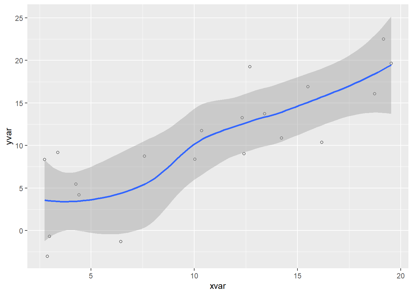 

Note that the code-fold: true parameter was added to the code chunk to hide the code by default (click the “Code” above to see the code).

Interactive Plots

You can also add interactive plots. For example:

library(dygraphs)
dygraph(nhtemp, main = "New Haven Temperatures") %>% 
  dyRangeSelector(dateWindow = c("1920-01-01", "1960-01-01"))

LaTeX Math

You can also include LaTeX math:

P\left(A=2\middle|\frac{A^2}{B}>4\right)