Theme Helpers

Overview

The quarto package includes helper functions for theming plotting and table packages.

The functions return theme objects or functions, which are applied differently depending on the package.

These are simple helper functions to get you started. Copy them if you to customize them further.

This vignette demonstrates adding background and foreground colors to outputs from each package using the theme_colors_* functions.

Please see light/dark renderings examples for examples using each supported package with dark mode, theme_brand_*, and renderings: [light, dark]

flextable

Demonstrates a flextable with green foreground and yellow background.

library(flextable)
library(quarto)

yellow_green_theme <- theme_colors_flextable("#e3e5a9", "#165b26")

ft <- flextable(airquality[ sample.int(10),])
ft <- add_header_row(ft,
  colwidths = c(4, 2),
  values = c("Air quality", "Time")
)
ft <- theme_vanilla(ft)
ft <- add_footer_lines(ft, "Daily air quality measurements in New York, May to September 1973.")
ft <- color(ft, part = "footer", color = "#666666")
ft <- set_caption(ft, caption = "New York Air Quality Measurements")

ft |> yellow_green_theme()

Air quality				Time
Ozone	Solar.R	Wind	Temp	Month	Day
41	190	7.4	67	5	1
36	118	8.0	72	5	2
28		14.9	66	5	6
12	149	12.6	74	5	3
18	313	11.5	62	5	4
8	19	20.1	61	5	9
	194	8.6	69	5	10
19	99	13.8	59	5	8
		14.3	56	5	5
23	299	8.6	65	5	7
Daily air quality measurements in New York, May to September 1973.

ggiraph

Demonstrates a ggiraph interactive plot with deep blue background and mauve foreground.

library(quarto)
library(ggplot2)
library(ggiraph)

blue_mauve_theme = theme_colors_ggplot2("#111038", "#E0B0FF")

cars <- ggplot(mtcars, aes(mpg, wt)) +
  geom_point_interactive(aes(colour = factor(cyl), tooltip = rownames(mtcars))) +
  scale_colour_manual(values = c("darkorange", "purple", "cyan4"))

girafe(ggobj = cars + blue_mauve_theme)

ggplot2

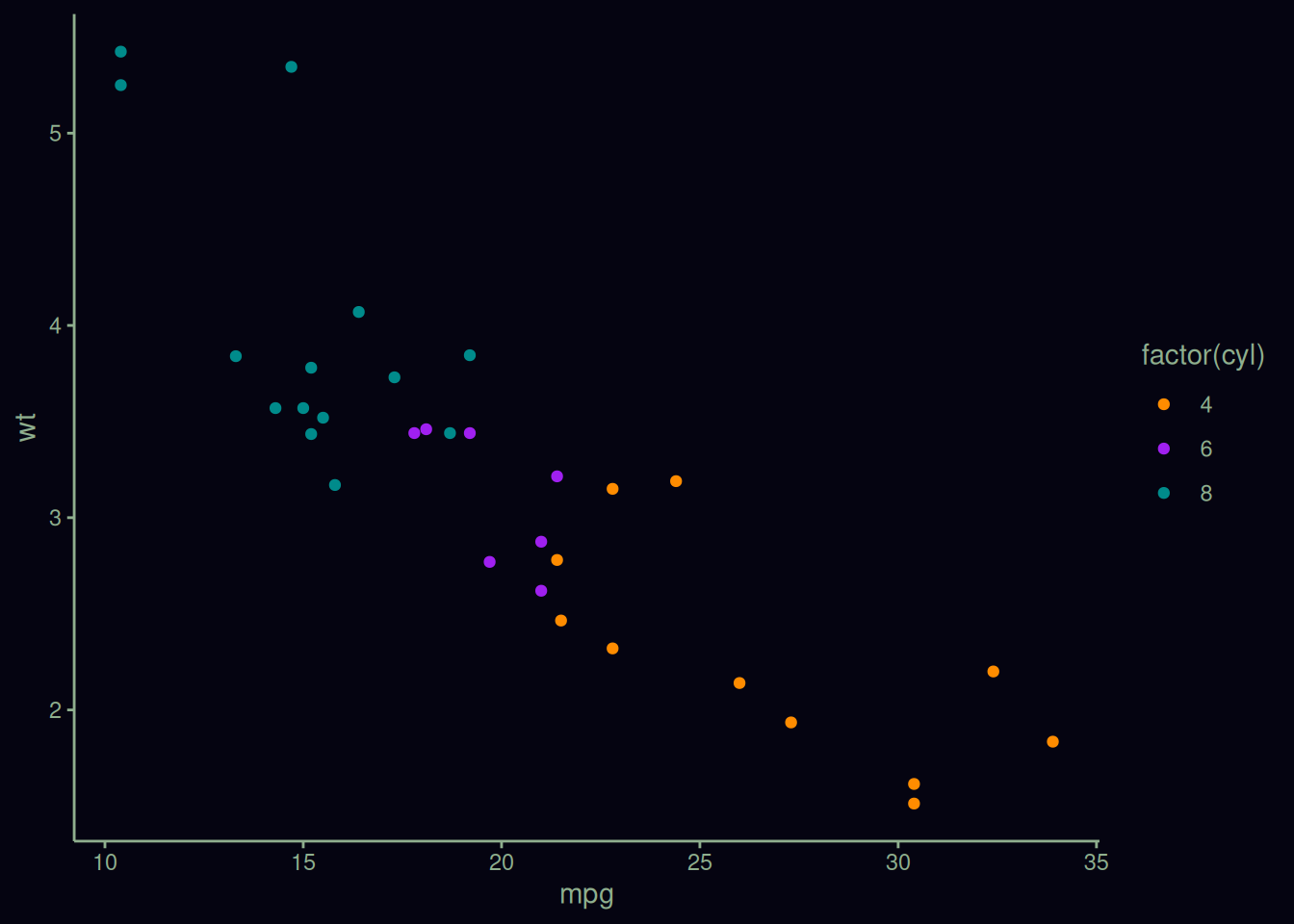
Demonstrates a ggplot2 plot with near-black background and green-grey foreground.

library(quarto)
library(ggplot2)

black_greyn <- theme_colors_ggplot2("#050411", "#8faf8e")

cars <- ggplot(mtcars, aes(mpg, wt)) +
  geom_point(aes(colour = factor(cyl))) +
  scale_colour_manual(values = c("darkorange", "purple", "cyan4"))

cars + black_greyn

gt

Demonstrates a gt table with light green background and black foreground.

library(gt)
library(quarto)
library(dplyr)

green_black_theme <- theme_colors_gt("#a5f7d6", "#020202")

islands_tbl <-
  tibble(
    name = names(islands),
    size = islands
  ) |>
  slice_max(size, n = 10)

gt(islands_tbl) |> green_black_theme()

name	size
Asia	16988
Africa	11506
North America	9390
South America	6795
Antarctica	5500
Europe	3745
Australia	2968
Greenland	840
New Guinea	306
Borneo	280

plotly

Demonstrates a heatmaply interactive heatmap with a dark green background background and light blue foreground.

library(quarto)
library(plotly)

green_blue_theme <- theme_colors_plotly("#293a0a", "#a5eff7")

fig <- plot_ly(iris, x = ~Species, y = ~Sepal.Width, type = "violin",
               box = list(visible = TRUE),
               meanline = list(visible = TRUE),
               points = "all")

fig |> green_blue_theme()

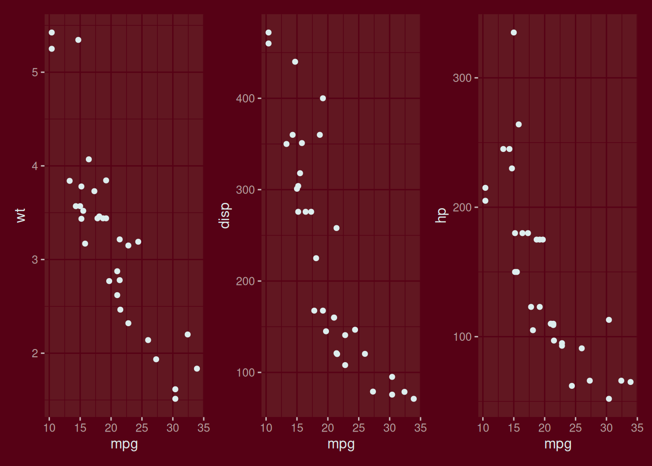
thematic

Demonstrates a patchwork plot with dark red background and light grey foreground.

library(ggplot2)
library(quarto)
library(patchwork)

darkred_grey_theme <- theme_colors_thematic("#560115", "#ddeeee");

#generate three scatterplots
plot1 <- ggplot(mtcars, aes(mpg, wt)) +
  geom_point()

plot2 <- ggplot(mtcars, aes(mpg, disp)) +
  geom_point()

plot3 <- ggplot(mtcars, aes(mpg, hp)) +
  geom_point()

#display all three scatterplots in same graphic
darkred_grey_theme()
plot1 + plot2 + plot3